class: center, middle, inverse, title-slide # Getting Started with R ### David Keyes // R for the Rest of Us --- layout: true <div class="dk-footer"> <span> <a href="https://rfortherestofus.com/" target="_blank">R for the Rest of Us </a> </span> </div> --- # Materials Slides and other materials from this session can be found at: ** bit.ly/benefitsofR** --- class: center, middle, dk-section-title background-image: url("images/installation.jpeg") # Installation --- ## Install R The first thing you need to do is download the R software. Go to the [Comprehensive R Archive Network (aka “CRAN”) website](https://cran.cnr.berkeley.edu/) and download the software for your operating system (Windows, Mac, or Linux). 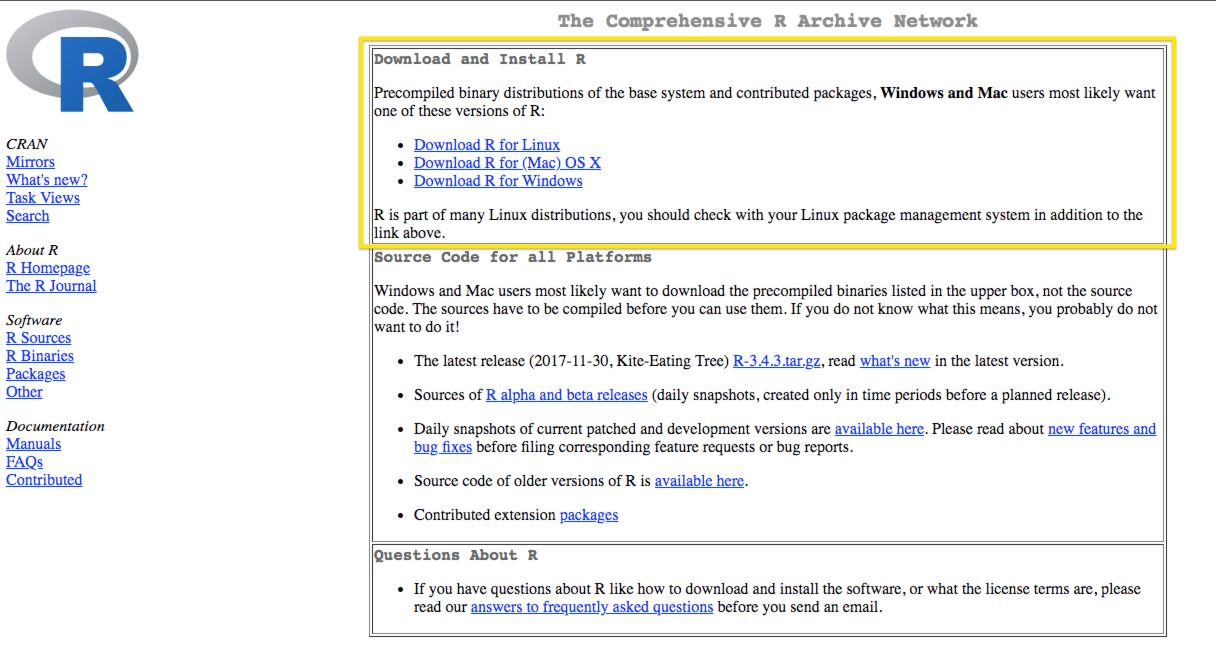 --- ### Working Directly in R 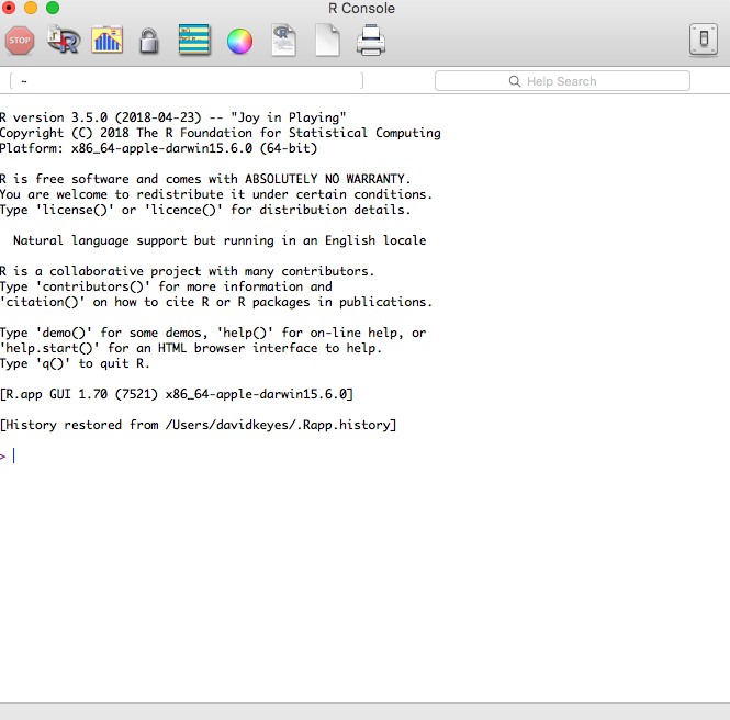 --- ## RStudio -- .center[ 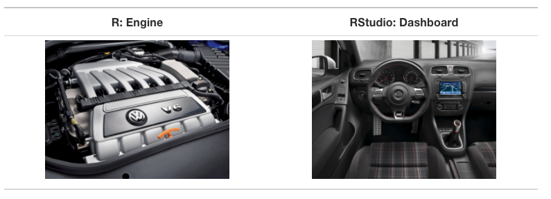 .small[Courtesy [Modern Dive](http://moderndive.com/2-getting-started.html#what-are-r-and-rstudio)] ] --- ### RStudio If you use RStudio, you’ll have a graphical user interface, the ability to see all of your stored information, and much more. 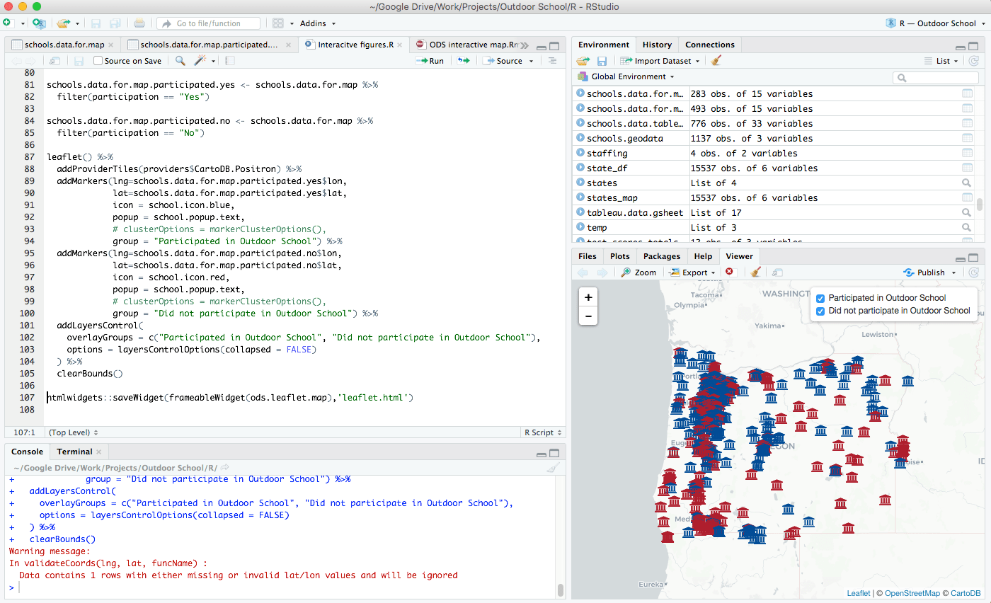 --- ### Download RStudio Download RStudio at the [RStudio website](https://www.rstudio.com/products/rstudio/download/#download). Ignore the various versions listed there. All you need is the latest version of RStudio Desktop. 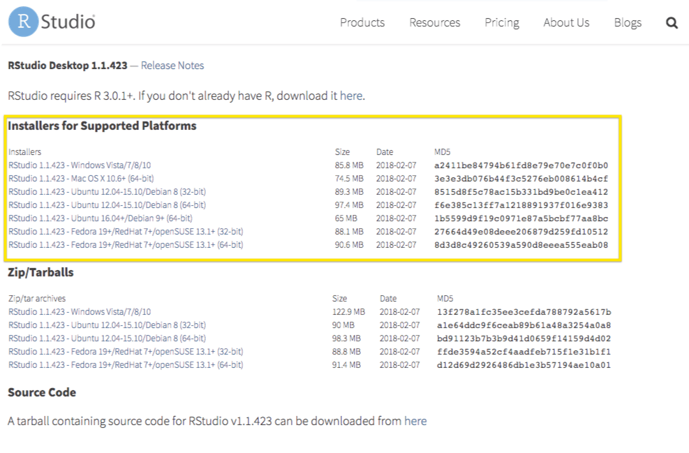 --- ### Tour of RStudio .center[ 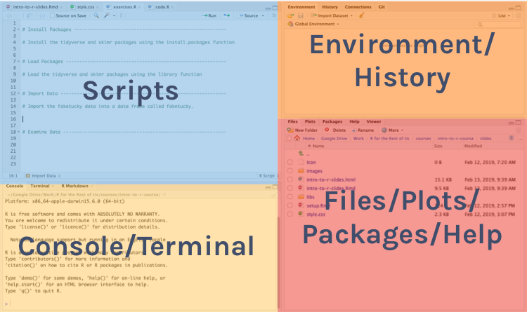 ] --- class: center, middle, dk-section-title background-image: url("images/packages.jpg") # Packages --- ## Packages Packages add functionality that is not present in base R. They're where much of the power of R is found. -- .center[ 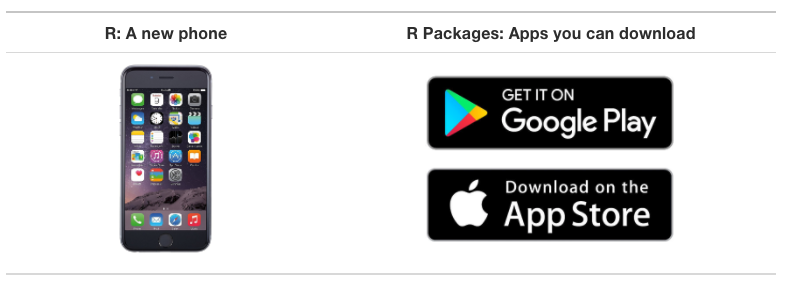 .small[Courtesy [Modern Dive](http://moderndive.com/2-getting-started.html#packages)] ] --- ## Packages We'll Use .pull-left[ .center[  ] ] .pull-right[ ### `tidyverse` The [`tidyverse`](https://tidyverse.org/) is a collection of packages. We'll use [`readr`](https://readr.tidyverse.org/) to import data. ] --- ## Packages We'll Use .pull-left[ ### `skimr` [`skimr`](https://github.com/ropensci/skimr) provides easy summary statistics. ] .pull-right[ .center[  ] ] --- ## Install Packages The syntax to install packages is as follows. ```r install.packages("tidyverse") install.packages("skimr") ``` The package name must be in quotes. -- .dk-highlight-box[ Packages should be installed **once per computer** (i.e. once you've installed a package, you don't need to do it again on the same computer). ] --- ## Load Packages To load packages, use the following syntax: ```r library(tidyverse) library(skimr) ``` Package names don't need to be quoted here (though they can be). -- .dk-highlight-box[ Packages should be loaded **once per session** (i.e. every time you start working in R, you need to load any packages you want to use). ] --- class: center, middle, dk-section-title background-image: url("images/data.jpg") # Import Data --- ## Import Data Let's read data from a CSV file. ```r faketucky <- read_csv("data/faketucky.csv") ``` We now have a data frame/tibble called `faketucky` that we can work with in R. ??? - Tibbles are ["modern data frames"](https://cran.r-project.org/web/packages/tibble/vignettes/tibble.html). The main difference for our purposes is that tibbles print much more nicely within R. - We'll use the terms tibble and data frame interchangeably. - For Excel files, try `read_excel` from the `readxl` package. - For SPSS files, try `read_sav` from the `haven` package. --- ## Where Does our Data Live? Data we have imported is available in the environment/history pane. .center[ 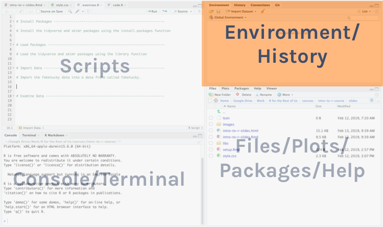 ] --- class: center, middle, dk-section-title background-image: url("images/glasses.jpeg") # Examine Our Data --- ## Examine Our Data There are many ways to look at our data. We'll talk about a few. --- ## `faketucky` If you type the name of your data frame (i.e. `faketucky`), R will output the following: ```r faketucky ``` -- ``` ## # A tibble: 57,855 x 9 ## student_id first_high_scho… school_district gender race_ethnicity ## <dbl> <chr> <chr> <chr> <chr> ## 1 1622 Jackson Jackson Male Multiple/Nati… ## 2 1877 Jackson Jackson Male White ## 3 1941 Jackson Jackson Male White ## 4 3442 Jackson Jackson Female White ## 5 4623 Jackson Jackson Male White ## 6 4913 Jackson Jackson Male White ## 7 5754 Jackson Jackson Male White ## 8 6293 Jackson Jackson Female White ## 9 7010 Jackson Jackson Male White ## 10 8343 Jackson Jackson Male White ## # … with 57,845 more rows, and 4 more variables: percent_absent <dbl>, ## # gpa <dbl>, act_reading_score <dbl>, act_math_score <dbl> ``` --- ## `View` `View` (note capital V) opens the RStudio viewer (or click on a data frame in the environment pane). ```r View(faketucky) ``` --- ## `skimr` The skimr package provides more detailed information about our data frame. It is also broken up by the type of variable. ```r skim(faketucky) ``` -- ``` ## Skim summary statistics ## n obs: 57855 ## n variables: 9 ## ## ── Variable type:character ───────────────────────────────────────────────────────────────────────────────── ## variable missing complete n min max empty n_unique ## first_high_school_attended 0 57855 57855 4 14 0 393 ## gender 14 57841 57855 4 6 0 2 ## race_ethnicity 794 57061 57855 5 24 0 5 ## school_district 0 57855 57855 4 13 0 171 ## ## ── Variable type:numeric ─────────────────────────────────────────────────────────────────────────────────── ## variable missing complete n mean sd p0 p25 ## act_math_score 14101 43754 57855 18.99 4.65 1 16 ## act_reading_score 14121 43734 57855 19.78 5.8 2 15 ## gpa 2185 55670 57855 2.59 0.87 0 2 ## percent_absent 111 57744 57855 8.78 16.02 0 3.26 ## student_id 0 57855 57855 55922.15 32332.71 1 27909.5 ## p50 p75 p100 hist ## 17 22 36 ▁▁▂▇▃▃▁▁ ## 19 23 36 ▁▁▅▇▆▃▂▁ ## 2.66 3.28 4 ▁▁▂▆▇▇▇▇ ## 6.27 11.3 3153 ▇▁▁▁▁▁▁▁ ## 56070 83872.5 111990 ▇▇▇▇▇▇▇▇ ```